02. Visualizing 2D linear transformations
In this post, we visualize how a linear operation encoded by a 2D matrix transforms a vector space. As an example, consider the matrix that transforms an arbitrary vector to a linear combination of the column vectors of :
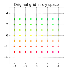
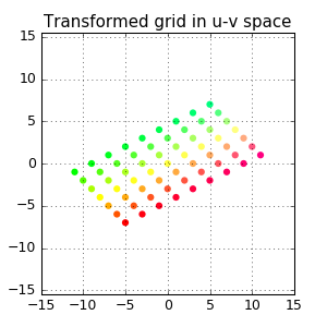
We can get a visual feel for this transformation by looking at a regular grid of points before and after the transformation:
But it’s fun to visualize this as an animation!
This post describes how to create such animations and uses them to visualize some common linear transforms. Click here to download the complete python script.
Strategy
- Create a rectangular array of points in x-y space.
- Map grid coordinates to colors that uniquely identify each point.
- Generate a series of intermediate transforms that will “smoothly” transition from the original grid to the transformed grid.
- Plot each of the intermediate transforms and save them as individual images.
- Stitch images into a gif.
Setup
Start a python shell and import libraries:
import numpy as np
import matplotlib as mpl
import matplotlib.pyplot as plt
Generate original and transformed grids
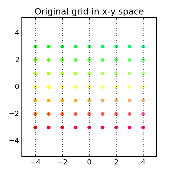
To construct a grid of points, we generate evenly spaced vectors along the x and y axes, and combine them together into a grid
# Create a grid of points in x-y space
xvals = np.linspace(-4, 4, 9)
yvals = np.linspace(-3, 3, 7)
xygrid = np.column_stack([[x, y] for x in xvals for y in yvals])
Here, the x-axis values span from -4 to 4 and the y-axis value span from -3 to 3. By stacking the x-y pairs columnwise, we generate a 2-by-n rectangular grid of points:
To generate the transformed grid, we perform a matrix multiplication:
# Apply linear transform
a = np.column_stack([[2, 1], [-1, 1]])
print(a)
uvgrid = np.dot(a, xygrid)
Plot grids
To plot the grid points, we will use the matplotlib function scatter that can apply a different color to each point. The following function transforms an (x,y) coordinate pair to an rgb color:
# This function assigns a unique color based on position
def colorizer(x, y):
    """
    Map x-y coordinates to a rgb color
    """
    r = min(1, 1-y/3)
    g = min(1, 1+y/3)
    b = 1/4 + x/16
    return (r, g, b)
We map this function to the x-y coordinates to generate an array of rgb color, and then plot the x-y grid points:
# Map grid coordinates to colors
colors = list(map(colorizer, xygrid[0], xygrid[1]))

# Plot grid points
plt.figure(figsize=(4, 4), facecolor="w")
plt.scatter(xygrid[0], xygrid[1], s=36, c=colors, edgecolor="none")
# Set axis limits
plt.grid(True)
plt.axis("equal")
plt.title("Original grid in x-y space")
which produces:
Similarly, we can plot the transformed grid:
# Plot transformed grid points
plt.figure(figsize=(4, 4), facecolor="w")
plt.scatter(uvgrid[0], uvgrid[1], s=36, c=colors, edgecolor="none")
plt.grid(True)
plt.axis("equal")
plt.title("Transformed grid in u-v space")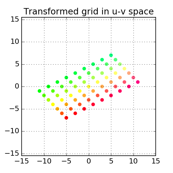
Generate intermediate transforms
To create the animated version, we need a series of intermediate grids that will smoothly transition from the original grid to the transformed grid. One way to achieve this is by constructing a series of 2-by-2 matrices that interpolate between the identity matrix and the target matrix . Supose we want to do this in n steps. Then the jth matrix in this sequence is: where . The matrix product computes grid coordinates for the jth intermediate transform. The following code block generates all the intermediate grids for a given target matrix, and returns the results in a 3d array:
# To animate the transform, we generate a series of intermediates
# Function to compute all intermediate transforms
def stepwise_transform(a, points, nsteps=30):
    '''
    Generate a series of intermediate transform for the matrix multiplication
      np.dot(a, points) # matrix multiplication
    starting with the identity matrix, where
      a: 2-by-2 matrix
      points: 2-by-n array of coordinates in x-y space

    Returns a (nsteps + 1)-by-2-by-n array
    '''
    # create empty array of the right size
    transgrid = np.zeros((nsteps+1,) + np.shape(points))
    # compute intermediate transforms
    for j in range(nsteps+1):
        intermediate = np.eye(2) + j/nsteps*(a - np.eye(2))
        transgrid[j] = np.dot(intermediate, points) # apply intermediate matrix transformation
    return transgrid

# Apply to x-y grid
steps = 30
transform = stepwise_transform(a, xygrid, nsteps=steps)
Plot intermediate transforms
Next we plot each of the intermediate grids on a common axis. To construct the animated version, we need to save each of these intermediate plots as an image file. The following code block defines a function that generates a series of image files with the filename frame-xx.png and saves them in a subdirectory. We apply this function to the array of intermediate grid coordinates that we generated above:
# Create a series of figures showing the intermediate transforms
def make_plots(transarray, color, outdir="png-frames", figuresize=(4,4), figuredpi=150):
    '''
    Generate a series of png images showing a linear transformation stepwise
    '''
    nsteps = transarray.shape[0]
    ndigits = len(str(nsteps)) # to determine filename padding
    maxval = np.abs(transarray.max()) # to set axis limits
    # create directory if necessary
    import os
    if not os.path.exists(outdir):
        os.makedirs(outdir)
    # create figure
    plt.ioff()
    fig = plt.figure(figsize=figuresize, facecolor="w")
    for j in range(nsteps): # plot individual frames
        plt.cla()
        plt.scatter(transarray[j,0], transarray[j,1], s=36, c=color, edgecolor="none")
        plt.xlim(1.1*np.array([-maxval, maxval]))
        plt.ylim(1.1*np.array([-maxval, maxval]))
        plt.grid(True)
        plt.draw()
        # save as png
        outfile = os.path.join(outdir, "frame-" + str(j+1).zfill(ndigits) + ".png")
        fig.savefig(outfile, dpi=figuredpi)
    plt.ion()

# Generate figures
make_plots(transform, colors, outdir="tmp")
Create animation
To stitch the image sequence into an animation, we use the ImageMagick, a cross-platform image manipulation library. The following code block performs this operation by making a system call to the convert script that is part of ImageMagick. (Note: This only works on linux or OS X and requires ImageMagick to be available at the command line)
# Convert to gif (works on linux/os-x, requires image-magick)
from subprocess import call
call("cd png-frames && convert -delay 10 frame-*.png ../animation.gif", shell=True)
# Optional: uncomment below clean up png files
#call("rm -f png-frames/*.png", shell=True)
which produces the following gif:
More examples
We can repeat this process for any 2d linear transformation. Below are some commmon linear transformation visualized as animations:
Rotation
Clockwise rotation by an angle is encoded by the rotation matrix
# Example 2: Rotation
theta = np.pi/3 # 60 degree clockwise rotation
a = np.column_stack([[np.cos(theta), np.sin(theta)], [-np.sin(theta), np.cos(theta)]])
print(a)
# Generate intermediates
transform = stepwise_transform(a, xygrid, nsteps=steps)
make_plots(transform, colors)
# see above to create gif
Shear
A shear matrix of the form stretches the grid along the x axis by an amount proportional to the y coordinate of a point.
# Example 3: Shear
a = np.column_stack([[1, 0], [2, 1]]) # shear along x-axis
print(a)
# Generate intermediates
transform = stepwise_transform(a, xygrid, nsteps=steps)
make_plots(transform, colors)
# see above to create gif
Permutation
The permutataion matrix interchanges the rows and columns:
# Example 4: Permutation
a = np.column_stack([[0, 1], [1, 0]])
print(a)
# Generate intermediates
transform = stepwise_transform(a, xygrid, nsteps=steps)
make_plots(transform, colors)
# see above to create gif
Projection
A projection onto the x-axis is encoded by the projection matrix .
# Example 5: Projection
a = np.column_stack([[1, 0], [0, 0]])
print(a)
# Generate intermediates
transform = stepwise_transform(a, xygrid, nsteps=steps)
make_plots(transform, colors)
# see above to create gif