01. Linear systems in 2D
Develop geometrical intuition for a 2D linear system
where is a 2-by-2 matrix, and and are 2-by-1 column vectors
Setup
Start a python shell and import libraries:
import numpy as np
import matplotlib as mpl
import matplotlib.pyplot as plt
# Change default color cycle (optional - may not work with older versions of matplotlib)
mpl.rcParams['axes.prop_cycle'] = mpl.cycler(color=["#377eb8","#ff7f00", "#4daf4a",
                                                    "#e41a1c", "#984ea3", "#a65628"])
Row picture
As a specific example, we consider the system
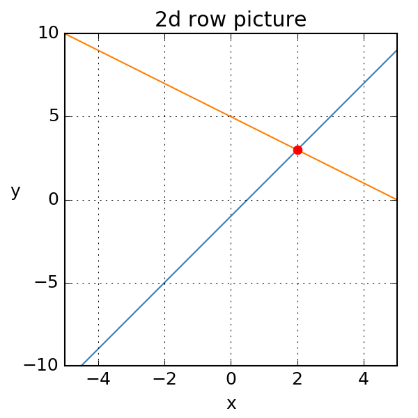
In the row picture, this system consists of following two linear equations:
Each equation above represents a straight line (of the form ). The following code block plots these lines. The solution is their intersection point (2, 3):
## Demo 1: Row picture
# 2x - y = 1
# x + y = 5

# generate points
x = np.array([-5, 5]) # We need only 2 points to draw a line
y1 = 2*x - 1
y2 = 5 - x

# plot the lines
plt.figure(figsize=(4, 4), facecolor="w")
plt.plot(x, y1, x, y2)
# show intersection point
plt.plot(2, 3, "ro", mec="r")
# add labels and gridlines
plt.title("2d row picture")
plt.xlabel("x")
plt.ylabel("y", rotation=0)
plt.xlim(x)
plt.ylim(ymin=-10)
plt.grid(True)
produces the following plot:

Column picture
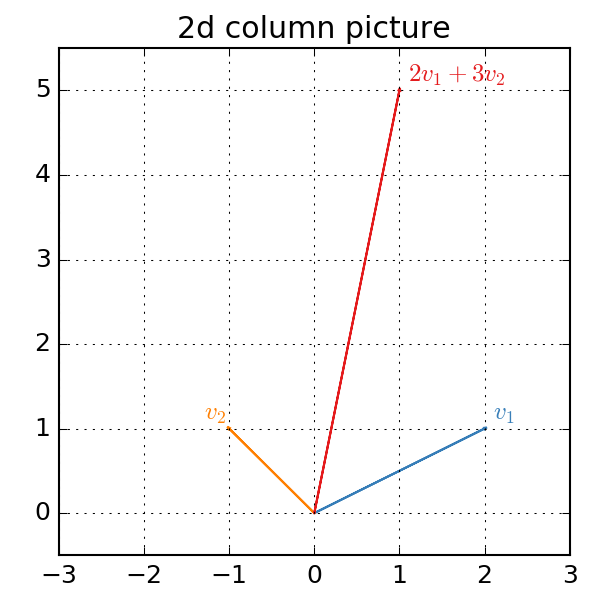
A different way to think about this problem is to view the operation as taking a linear combination of the columns of and ask what is is the correct linear combination that gives us . In other words, for what values of and do we get:
The next code block plots the two column vectors and the correct linear combination:
## Demo 2: Column picture of matrix multiplication
# Create vectors and the correct linear combination
v1 = np.array([2, 1])
v2 = np.array([-1, 1])
lc = 2*v1 + 3*v2
# plot all three vectors
plt.clf()
plt.arrow(0, 0, v1[0], v1[1], color="#377eb8")
plt.arrow(0, 0, v2[0], v2[1], color="#ff7f00")
plt.arrow(0, 0, lc[0], lc[1], color="#e41a1c")
# add title labels, etc.
plt.title("2d column picture")
plt.text(2.1, 1.1, r"$v_1$", color="#377eb8")
plt.text(-1.3, 1.1, r"$v_2$", color="#ff7f00")
plt.text(1.1, 5.1, r"$2 v_1 + 3 v_2$", color="#e41a1c")
plt.xlim((-3, 3))
plt.ylim((-0.5, 5.5))
plt.grid(True)
Visualizing the column space
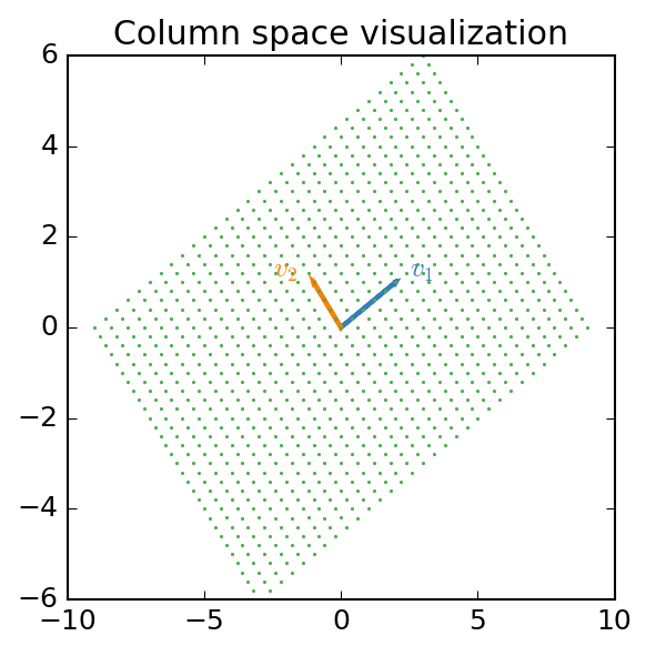
The column space of a matrix is the span of the column vectors, i.e. the set of all possible linear combinations of the columns.
# Demo 3: Visualizing how linear combinations of two vectors span a plane
v1 = np.array([2, 1])
v2 = np.array([-1, 1])
a = np.column_stack((v1, v2))
xvals = np.linspace(-3, 3, 31)
yvals = np.linspace(-3, 3, 31)
grid = np.column_stack([[x, y] for x in xvals for y in yvals])
lc = np.dot(a, grid)

# plot linear combinations
plt.clf()
plt.plot(lc[0], lc[1], ".", color="#4daf4a", ms=2)
plt.arrow(0, 0, v1[0], v1[1], color="#377eb8", lw=2)
plt.arrow(0, 0, v2[0], v2[1], color="#ff7f00", lw=2)
plt.title("Column space visualization")
The green dots in the plot below show the specific linear combinations we generated from the two column vectors

Solving a linear system
How to solve the linear system for given and
# Demo 4: Solving the linear system
# Solve for 1 linear combination
a = np.array([[2, -1], [1, 1]])
b = np.array([1, 5])
sol = np.linalg.solve(a, b)
print(sol)